Module 0: Introduction to Scientific Computing¶

This section will provide the necessary background in Python programming needed to complete the rest of this course. While most models can be implemented using a number of different possible programming languages, we will be using Python as our language of choice throughout this course. Python is a widely used, open-source programming language with a wide variety of community-built packages for scientific use (numerical methods, data analysis, plotting and visualization, etc.)

0.1 Mathematical Operations, Defining Variables, and Plotting¶

Adapted from Mark Bakker Delft University of Technology
View this section as an executable Jupyter Notebook: https://tinyurl.com/y5s5ypvm

The google collaboratory environment provides you with a cloud-hosted jupyter notebook environment. This enables you to use and run python code that we provide. We know that this is not a programming course so we keep the coding burden very light. We make extensive use of text fields like this to ‘scaffold’ the upcoming exercise.

Note: If you decide to use the notebooks online to follow along, we recommend using Google Chrome to make sure all the functions work smoothly. Other browsers should work, but if you encounter problems with formatting or cells not running properly, try running the notebook again in Chrome as your first debugging step.

In this section, we are going to go over the basics of defining variables and plotting things. For our first example, we will demonstrate how to use Python as a simple calculator. As we work through the following examples, feel free to use code commenting to take notes on what the different parts of each command do. You can save the notebook linked above to your own google drive and always have your own copy for future reference.

The cell below shows the sytax for basic multiplication in Python. When running this in a Python shell, or when executing a cell in your Colab notebook, the Python interpreter will output a value of 12.

6 * 2

Python is not fussy about spaces. Look at the code in the following cell…even though the 6 and the 2 are much further apart, it will still run as though there were no extra spaces.

6   *                        2

If you want to “comment out” a line of code that you want to leave in your document but that you don’t want to run, you can do that by placing a “#” at the start of the line. You can comment out blocks of code by adding the “#” to the start of each line in the block. Many code editors will have functions that allow you to comment out large blocks of highlighted text with a single command.

# This is a comment in Python. It will not be run by the program.
# The value output from running the command below should be 12
6 * 2

You can also add comments directly in the code if you want to add some details to what that line of code does. In the example below you can see a comment line that does not affect the code but it just to help understand the code. Good commenting is good coding practice!

6 * 2 # This line calculates the product of 6 and 2

Defining Variables.

To do scientific computing we will need to store the values within variables. look at the cell below. It can not run because there is a question-mark where the value for b should be.

We will often use this approach as a fill-in-the-blank exercise to help get you started with a code. However, most of the problems we give are a little bit harder than this.

Modify the code below to assign a value of 2 to the variable b

a = 6
b = 2
a * b

Both a and b are now variables. Each variable has a type. In this case, they are both integers (whole numbers). To write the value of a variable to the screen, use the print function (the last statement of a code cell is automatically printed to the screen if it is not stored in a variable, as was shown above)

print(a)
print(b)
print(a * b)
print(a / b)

You can add some text to the print function by putting the text between quotes (either single or double quotes work as long as you use the same at the beginning and end), and separate the text string and the variable by a comma

print('the value of a is', a)

A variable can be raised to a power by using ** (a hat ^, as used in some other languages, doesn’t work).

a ** b

Exercise 0.1.1a: First Python code¶

Compute the value of the polynomial \(y=ax^2+bx+c\) at \(x=-2\), \(x=0\), and \(x=2.1\) using \(a=1\), \(b=1\), \(c=-6\) and print the results to the screen.

Division¶

Division works as well

print('1/3 gives', 1 / 3)

(Note for Python 2 users: 1/3 gives zero in Python 2, as the division of two integers returned an integer in Python 2). The above print statement looks pretty ugly with 16 values of 3 in a row. A better and more readable way to print both text and the value of variable to the screen is to use what are called f-strings. f-strings allow you to insert the value of a variable anywhere in the text by surrounding it with braces {}. The entire text string needs to be between quotes and be preceded by the letter f

a = 1
b = 3
c = a / b
print(f'{a} divided by {b} gives {c}')

The complete syntax between braces is {variable:width.precision}. When width and precision are not specified, Python will use all digits and figure out the width for you. If you want a floating point number with 3 decimals, you specify the number of digits (3) followed by the letter f for floating point (you can still let Python figure out the width by not specifying it). If you prefer exponent (scientific) notation, replace the f by an e. The text after the # is a comment in the code. Any text on the line after the # is ignored by Python.

print(f'{a} divided by {b} gives {c:.3f}') # three decimal places
print(f'{a} divided by {b} gives {c:10.3f}') # width 10 and three decimal places
print(f'{a} divided by {b} gives {c:.3e}') # three decimal places scientific notation

Exercise 0.1.1b:First Python code using f-strings¶

Compute the value of the polynomial \(y=ax^2+bx+c\) at \(x=-2\), \(x=0\), and \(x=2.1\) using \(a=1\), \(b=1\), \(c=-6\) and print the results to the screen using f-strings and 2 decimal places.

More on variables¶

Once you have created a variable in a Python session, it will remain in memory, so you can use it in other cells as well. For example, the variables a and b, which were defined two code cells above in this Notebook, still exist.

print(f'the value of a is: {a}')
print(f'the value of b is: {b}')

The user (in this case: you!) decides the order in which code blocks are executed. For example, In [6] means that it is the sixth execution of a code block. If you change the same code block and run it again, it will get number 7. If you define the variable a in code block 7, it will overwrite the value of a defined in a previous code block.

Variable names may be as long as you like (you gotta do the typing though). Selecting descriptive names aids in understanding the code. Variable names cannot have spaces, nor can they start with a number. And variable names are case sensitive. So the variable myvariable is not the same as the variable MyVariable. The name of a variable may be anything you want, except for reserved words in the Python language. For example, it is not possible to create a variable for = 7, as for is a reserved word. You will learn many of the reserved words when we continue; they are colored bold green when you type them in the Notebook.

Basic plotting and a first array¶

Plotting is not part of standard Python, but a nice package exist to create pretty graphics (and ugly ones, if you want). A package is a library of functions for a specific set of tasks. There are many Python packages and we will use several of them. The graphics package we use is called matplotlib. To be able to use the plotting functions in matplotlib we have to import it. We will learn several different ways of importing packages. For now, we import the plotting part of matplotlib and call it plt. Before we import matplotlib, we tell the Jupyter Notebook to show any graphs inside this Notebook and not in a separate window (more on these commands later).

%matplotlib inline
import matplotlib.pyplot as plt

Packages only have to be imported once in a Python session. After the above import statement, any plotting function may be called from any code cell as plt.function. For example

plt.plot([1, 2, 4, 2])

Let’s try to plot \(y\) vs \(x\) for \(x\) going from \(-4\) to \(+4\) for the polynomial \(y=ax^2+bx+c\) with \(a=1\), \(b=1\), \(c=-6\). To do that, we need to evaluate \(y\) at a bunch of points. A sequence of values of the same type is called an array (for example an array of integers or floats). Array functionality is available in the package numpy. Let’s import numpy and call it np, so that any function in the numpy package may be called as np.function.

import numpy as np

To create an array x consisting of, for example, 5 equally spaced points between -4 and 4, use the linspace command

x = np.linspace(-4, 4, 5)
print(x)

In the above cell, x is an array of 5 floats (-4. is a float, -4 is an integer). If you type np.linspace and then an opening parenthesis like:

np.linspace(

and then hit [shift-tab] a little help box pops up to explain the input arguments of the function. When you click on the + sign, you can scroll through all the documentation of the linspace function. Click on the x sign to remove the help box. Let’s plot \(y\) using 100 \(x\) values from \(-4\) to \(+4\).

a = 1
b = 1
c = -6
x = np.linspace(-4, 4, 100)
y = a * x ** 2 + b * x + c  # Compute y for all x values
plt.plot(x, y);

Note that one hundred y values are computed in the simple line y = a * x ** 2 + b * x + c. Python treats arrays in the same fashion as it treats regular variables when you perform mathematical operations. The math is simply applied to every value in the array (and it runs much faster than when you would do every calculation separately).

You may wonder what the statement [<matplotlib.lines.Line2D at 0x30990b0>] is (the numbers on your machine may look different). This is actually a handle to the line that is created with the last command in the code block (in this case plt.plot(x, y)). Remember: the result of the last line in a code cell is printed to the screen, unless it is stored in a variable. You can tell the Notebook not to print this to the screen by putting a semicolon after the last command in the code block (so type plot(x, y);). We will learn later on that it may also be useful to store this handle in a variable.

The plot function can take many arguments. Looking at the help box of the plot function, by typing plt.plot( and then shift-tab, gives you a lot of help. Typing plt.plot? gives a new scrollable subwindow at the bottom of the notebook, showing the documentation on plot. Click the x in the upper right hand corner to close the subwindow again.

In short, plot can be used with one argument as plot(y), which plots y values along the vertical axis and enumerates the horizontal axis starting at 0. plot(x, y) plots y vs x, and plot(x, y, formatstring) plots y vs x using colors and markers defined in formatstring, which can be a lot of things. It can be used to define the color, for example 'b' for blue, 'r' for red, and 'g' for green. Or it can be used to define the linetype '-' for line, '--' for dashed, ':' for dots. Or you can define markers, for example 'o' for circles and 's' for squares. You can even combine them: 'r--' gives a red dashed line, while 'go' gives green circular markers.

If that isn’t enough, plot takes a large number of keyword arguments. A keyword argument is an optional argument that may be added to a function. The syntax is function(keyword1=value1, keyword2=value2), etc. For example, to plot a line with width 6 (the default is 1), type

plt.plot([1, 2, 3], [2, 4, 3], linewidth=6);

Keyword arguments should come after regular arguments. plot(linewidth=6, [1, 2, 3], [2, 4, 3]) gives an error.

Names may be added along the axes with the xlabel and ylabel functions, e.g., plt.xlabel('this is the x-axis'). Note that both functions take a string as argument. A title can be added to the figure with the plt.title command. Multiple curves can be added to the same figure by giving multiple plotting commands in the same code cell. They are automatically added to the same figure.

New figure and figure size¶

Whenever you give a plotting statement in a code cell, a figure with a default size is automatically created, and all subsequent plotting statements in the code cell are added to the same figure. If you want a different size of the figure, you can create a figure first with the desired figure size using the plt.figure(figsize=(width, height)) syntax. Any subsequent plotting statement in the code cell is then added to the figure. You can even create a second figure (or third or fourth…).

plt.figure(figsize=(10, 3))
plt.plot([1, 2, 3], [2, 4, 3], linewidth=6)
plt.title('very wide figure')
plt.figure()  # new figure of default size
plt.plot([1, 2, 3], [1, 3, 1], 'r')
plt.title('second figure');

Exercise 0.1.2a: First graph¶

Plot \(y=(x+2)(x-1)(x-2)\) for \(x\) going from \(-3\) to \(+3\) using a dashed red line. On the same figure, plot a blue circle for every point where \(y\) equals zero. Set the size of the markers to 10 (you may need to read the help of plt.plot to find out how to do that). Label the axes as ‘x-axis’ and ‘y-axis’. Add the title ‘First nice Python figure of Your Name’, where you enter your own name.

Style¶

As was already mentioned above, good coding style is important. It makes the code easier to read so that it is much easier to find errors and bugs. For example, consider the code below, which recreates the graph we produced earlier (with a wider line), but now there are no additional spaces inserted

a=1
b=1
c=-6
x=np.linspace(-4,4,100)
y=a*x**2+b*x+c#Compute y for all x values
plt.plot(x,y,linewidth=3)

The code in the previous code cell is difficult to read. Good style includes at least the following: * spaces around every mathematical symbol (=, +, -, *, /), but not needed around ** * spaces between arguments of a function * no spaces around an equal sign for a keyword argument (so linewidth=3 is correct) * one space after every comma * one space after each # * two spaces before a # when it follows a Python statement * no space between the function name and the list of arguments. So plt.plot(x, y) is good style, and plt.plot (x, y) is not good style.

These rules are (a very small part of) the official Python style guide called PEP8. When these rules are applied, the code is as follows:

a = 1
b = 1
c = -6
x = np.linspace(-4, 4, 100)
y = a * x**2 + b * x + c  # Compute y for all x values
plt.plot(x, y, linewidth=3)

Exercise 0.1.2b: First graph revisited¶

Go back to your Exercise 2 and apply correct style.

0.2: Loops and Logic¶

Adapted from Mark Bakker Delft University of Technology
View this section as an executable Jupyter Notebook: https://tinyurl.com/r64mryn

In scientific computing we rely on the following packages so lets import them by running the following commands

import numpy as np
import matplotlib.pyplot as plt

For Loops in python are very similar to for loops in other languages.

Execute the following command to see how the variable i is updated each time the command ‘loops’ through.

Also note that the for comand ends with a : and the commands inside the loop are indented.

As we work through the following examples please use code commenting to take notes on what the different parts of each command do. You can save this notebook to your own google drive and always have this as a reference for the rest of the course.

for i in [0, 1, 2, 3, 4]:
    print('Hello world, the value of i is', i)

Hello world, the value of i is 0
Hello world, the value of i is 1
Hello world, the value of i is 2
Hello world, the value of i is 3
Hello world, the value of i is 4

You can use multiple commands inside the loop as long as they are all indented. Commands that are not indented will be executed after the conclusion of the loop as in the example below

for x in [0, 1, 2, 3]:
    xsquared = x ** 2
    print('x, xsquare', x, xsquared)
print('We are done with the loop')

x, xsquare 0 0
x, xsquare 1 1
x, xsquare 2 4
x, xsquare 3 9
We are done with the loop

To save the effort of listing each variable value for your looped variable you can use the range argument to generate the values. Note that in python you typically start counting from 0 not from 1 so range(7) produces a list of 7 numbers from 0 to 6

for i in range(7):
    print('the value of i is:', i)

the value of i is: 0
the value of i is: 1
the value of i is: 2
the value of i is: 3
the value of i is: 4
the value of i is: 5
the value of i is: 6

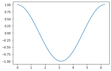
For loops can be useful for conducting a set of calculations that you might use in a graph. Examine the following example

x = np.linspace(0, 2 * np.pi, 100)
y = np.zeros_like(x)  # similar to zeros(shape(x))
for i in range(len(x)):
    y[i] = np.cos(x[i])
plt.plot(x, y);

Note, that the variables in a for loop do not have to be numbers, they can be calculated values. They can even be names. Execute the following commands to see how to use text variables.

for x in ['Dr. Umulis', 'Dr. Pienaar']:
  print('One of my favorite professors is '+str(x))

One of my favorite professors is Dr. Umulis
One of my favorite professors is Dr. Pienaar

Also note that you can use your index variable to communicate multiple values to your for loop. This can be useful in solving complex systems of equations. Explore the following example with your group

months = ['January', 'February', 'March', 'April',\
          'May','June', 'July', 'August', 'September',\
          'October', 'November', 'December']
days = [31, 28, 31, 30, 31, 30, 31, 31, 30, 31, 30, 31]
for i in range(12):
    print('The number of days in '+str(months[i])+' is ' +str(days[i]))

Exercises

Exercise 0.2.1: Printing with Loops¶

Using the above examples, build a loop that prints the names of your five favorite bands. Click the “Begin” button below to try it yourself.

[Interactive Functionality coming soon]

0.3: Making Reusable Code — Defining Functions¶

Adapted from Mark Bakker Delft University of Technology
View this section as an executable Jupyter Notebook: https://tinyurl.com/rvhzpuq

In scientific computing we rely on the following packages so lets import them by running the following commands

import numpy as np
import matplotlib.pyplot as plt

Defining Functions in python is once again very similar to MatLab.

Defining a function is useful because it saves you from having to rewrite large loops over and over again.

To define a new function, use the command def followed by the name of your function and then parentheses sorrounding the arguments or inputs into the function. T as follows:

def function_name(Argument1, Argument2):

After the colon the commands within the function are indented (just as in for loops). The final command of the function should be return followed by the output variable.

Examine the example below.

Reminder: As we work through the following examples please use code commenting to take notes on what the different parts of each command do. You can save this notebook to your own google drive and always have this as a reference for the rest of the course.

def MyFirstFunction(a, b, c):
  Output = a**2 + b**3 - c**.5
  return Output

# Remember that exponents in python are defined by ** not by the ^ symbol

Note that simply defining the function does not result in any output. We have to call the function and supply the input arguments (in this case, a, b and c)

MyFirstFunction(6,2,8)
MyFirstFunction(5,2,1)

32.0

Note that only the most recent call of the function is returned here. To see the output of each time you call the function we need to explicitly capture the output and ask the notebook to print the function, as shown below

CaptureOuput1 = MyFirstFunction(1,5,3)
print('The Output of the first function call is '+str(CaptureOuput1))
CaptureOuput2 = MyFirstFunction(3,6,11)
print('The Output of the second function call is '+str(CaptureOuput2))

The Output of the first function call is 124.26794919243112
The Output of the second function call is 221.6833752096446

Note that you can have functions that return multiple values

def testfunction(a, b):
  hypotenus = (a**2 + b**2)**.5
  perimeter = a + b + hypotenus
  return (hypotenus, perimeter)
z = 6;
w = 8;
CaptureOutput = testfunction(z,w)
print('a right triangle with sides of '+str(z)+", and "+str(w)+", will have a hypotenus of "+str(CaptureOutput[0])+ ", and a perimeter of "+str(CaptureOutput[1]))

a right triangle with sides of 6, and 8, will have a hypotenus of 10.0, and a perimeter of 24.0

Exercise 0.3.1: Calling Custom Functions¶

Using the examples above, define a function for the following equation

f(x)=3^α * cos(x)

and then call the function with input arguments α = 4 and x = 8

Note: you need to google the numpy command for calculating cos

the expected answer is -11.785502738497696

import numpy as np
def exercise(a, x):

advanced can write a function that includes a for loop.

0.4: Answers for the exercises¶

Answer to Exercise 0.1.1a:

a = 1
b = 1
c = -6
x = -2
y = a * x ** 2 + b * x + c
print('y evaluated at x = -2 is', y)
x = 0
y = a * x ** 2 + b * x + c
print('y evaluated at x = 0 is', y)
x = 2.1
y = a * x ** 2 + b * x + c
print('y evaluated at x = 2 is', y)

# Errored Code
a = 1
b = 1
c = -6
x = -2
y = a * x ** 2 + b * x + c
print('y evaluated at x = -2 is', y)
x = 0
a = 2
y = a * x ** 2 + b * x + c
print('y evaluated at x = 0 is', y)
x = 2.1
y = a * x ** 2 + b * x + c
print('y evaluated at x = 2 is', y)

Back to Exercise 1a

Answer to Exercise 0.1.1b:

a = 1
b = 1
c = -6
x = -2
y = a * x ** 2 + b * x + c
print(f'y evaluated at x = {x} is {y}')
x = 0
y = a * x ** 2 + b * x + c
print(f'y evaluated at x = {x} is {y}')
x = 2.1
y = a * x ** 2 + b * x + c
print(f'y evaluated at x = {x} is {y:.2f}')

Back to Exercise 1b

Answer to Exercise 0.1.2

x = np.linspace(-3, 3, 100)
y = (x + 2) * (x - 1) * (x - 2)
plt.plot(x, y, 'r--')
plt.plot([-2, 1, 2], [0, 0, 0], 'bo', markersize=10)
plt.xlabel('x-axis')
plt.ylabel('y-axis')
plt.title('First Python Figure of Mark Bakker');

Back to Exercise 0.1.2

Answer to Exercise 0.1.3

holland = np.loadtxt('/content/ThermoData/holland_temperature.dat')
newyork= np.loadtxt('/content/ThermoData/newyork_temperature.dat')
beijing = np.loadtxt('/content/ThermoData/beijing_temperature.dat')
plt.plot(np.linspace(1, 12, 12), holland)
plt.plot(np.linspace(1, 12, 12), newyork)
plt.plot(np.linspace(1, 12, 12), beijing)
plt.xlabel('Number of the month')
plt.ylabel('Mean monthly temperature (Celcius)')
plt.xticks(np.linspace(1, 12, 12))
plt.legend(['Holland','New York','Beijing'], loc='best');

# Errored Code
holland = np.loadtxt('/content/ThermoData/holland_temperature.dat')
newyork= np.loadtxt('/content/ThermoData/newyork_temperature.dat')
beijing = np.loadtxt('/content/ThermoData/beijing_temperature.dat')
plt.plot(np.linspace(1, 10, 10), holland)
plt.plot(np.linspace(1, 10, 10), newyork)
plt.plot(np.linspace(1, 12, 12), beijing)
plt.xlabel('Number of the month')
plt.ylabel('Mean monthly temperature (Celcius)')
plt.xticks(np.linspace(1, 10, 10))
plt.legend(['Holland','New York'], loc='best');

Back to Exercise 0.1.3

Answer to Exercise 0.1.4

air = np.loadtxt('/content/ThermoData/holland_temperature.dat')
sea = np.loadtxt('/content/ThermoData/holland_seawater.dat')
plt.subplot(211)
plt.plot(air, 'b', label='air temp')
plt.plot(sea, 'r', label='sea temp')
plt.legend(loc='best')
plt.ylabel('temp (Celcius)')
plt.xlim(0, 11)
plt.xticks([])
plt.subplot(212)
plt.plot(air-sea, 'ko')
plt.xticks(np.linspace(0, 11, 12),
           ['jan','feb','mar','apr','may','jun','jul','aug','sep','oct','nov','dec'])
plt.xlim(0, 11)
plt.ylabel('air - sea temp (Celcius)');

Back to Exercise 0.1.4

Answer to Exercise 0.1.5

gold = [46, 38, 29, 24, 13, 11, 11, 8, 8, 7, 107]
countries = ['USA', 'CHN', 'GBR', 'RUS', 'KOR', 'GER', 'FRA', 'ITA', 'HUN', 'AUS', 'OTHER']
plt.pie(gold, labels = countries, colors = ['Gold', 'MediumBlue', 'SpringGreen', 'BlueViolet'])
plt.axis('equal');

gold = [46, 38, 29, 24, 13, 11, 11, 8, 8, 7, 107]
countries = ['USA', 'CHN', 'GBR', 'RUS', 'KOR', 'GER', 'FRA', 'ITA', 'HUN', 'AUS', 'Other']
plt.pie(gold, labels = countries, colors = ['Gold', 'MediumBlue', 'SpringGreen', 'BlueViolet'])
plt.legend('USA', 'CHN')
plt.axis('equal');

Back to Exercise 0.1.5

Answer to Exercise 0.1.6

air = np.loadtxt('/content/ThermoData/holland_temperature.dat')
sea = np.loadtxt('/content/ThermoData/holland_seawater.dat')
plt.fill_between(range(1, 13), air, color='b', alpha=0.3)
plt.fill_between(range(1, 13), sea, color='r', alpha=0.3)
plt.xticks(np.linspace(0, 11, 12), ['jan', 'feb', 'mar', 'apr',\
           'may', 'jun', 'jul', 'aug', 'sep', ' oct', 'nov', 'dec'])
plt.xlim(1, 12)
plt.ylim(0, 20)
plt.xlabel('Month')
plt.ylabel('Temperature (Celcius)');

Back to Exercise 0.1.6